After over one year I finally found time and leisure to write my next article. This time about finetuning AlexNet in pure TensorFlow 1.0. “AlexNet?” you might say, “So 2012’ish!” you might say. Well here are some reasons why I thought it’s worth doing anyway:
- Albeit there exist many How-To’s, most of the newer once are covering finetuning VGG or Inception Models and not AlexNet. Although the idea behind finetuning is the same, the major difference is, that Tensorflow (as well as Keras) already ship with VGG or Inception classes and include the weights (pretrained on ImageNet). For the AlexNet model, we have to do a bit more on our own.
- Another reason is that for a lot of my personal projects AlexNet works quite well and there is no reason to switch to any of the more heavy-weight models to gain probably another .5% accuracy boost. As the models get deeper they naturally need more computational time, which in some projects I can’t afford.
- In the past, I used mainly Caffe to finetune convolutional networks. But to be honest, I found it quite cumbersome (e.g. model definition via .prototxt, the model structure with blobs…) to work with Caffe. After some time with Keras, I recently switched to pure TensorFlow and now I want to be able to finetune the same network as previously, but using just TensorFlow.
- Well and I think the main reason for this article is that working on a project like this, helps me to better understand TensorFlow in general.
Disclaimer
After finishing to write this article I ended up having written another very long post. Basically it is divided into two parts: In the first part I created a class to define the model graph of AlexNet together with a function to load the pretrained weights and in the second part how to actually use this class to finetune AlexNet on a new dataset. Although I recommend reading the first part, click here to skip the first part and go directly on how to finetune AlexNet.
And next: This is not an introduction neither to TensorFlow nor to finetuning or convolutional networks in general. I’ll explain most of the steps you need to do, but basic knowledge of TensorFlow and machine/deep learning is required to fully understand everything.
Getting the pretrained weights
Unlike VGG or Inception, TensorFlow doesn’t ship with a pretrained AlexNet. Caffe does, but it’s not to trivial to convert the weights manually in a structure usable by TensorFlow. Luckily Caffe to TensorFlow exists, a small conversion tool, to translate any *prototxt model definition from caffe to python code and a TensorFlow model, as well as conversion of the weights. I tried it on my own and it works pretty straight forward. Anyway, here you can download the already converted weights.
Model structure
To start finetune AlexNet, we first have to create the so-called “Graph of the Model”. This is the same thing I defined for BatchNormalization in my last blog post but for the entire model. But don’t worry, we don’t have to do everything manually. Let’s first look onto the model structure as shown in the original paper:
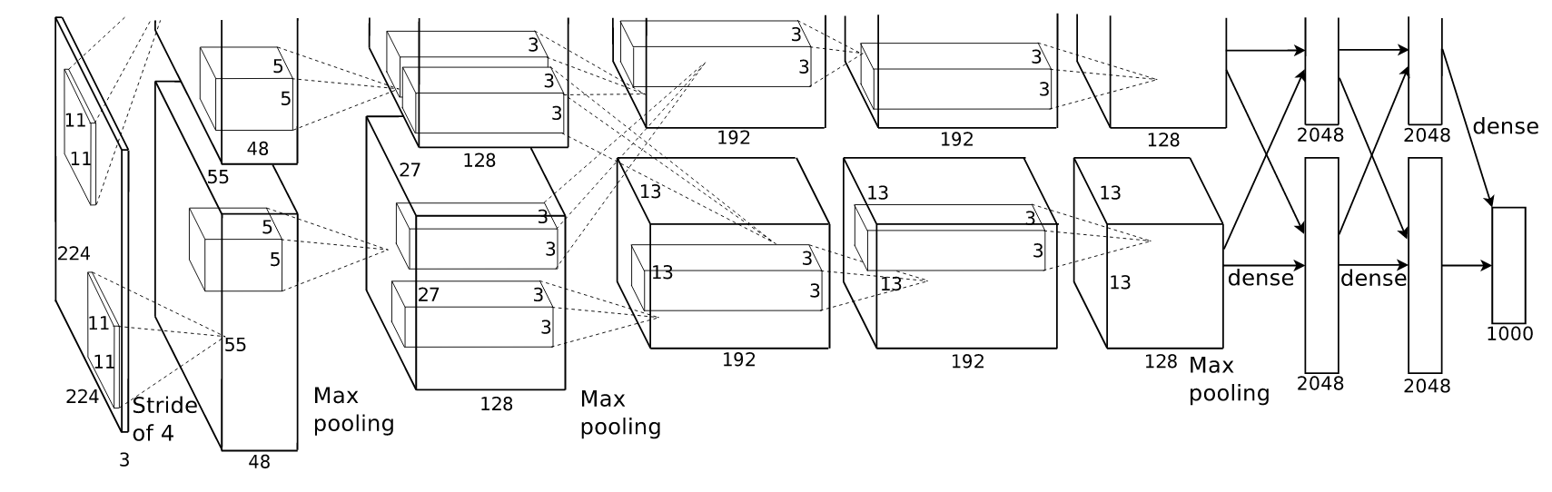
Architecture of AlexNet, as shown in the original paper (link above).
Noteworthy are the splitting of some of the convolutional layer (layer two, four and five). It has been used to split up the computation between two GPUs (I guess because GPUs weren’t so strong at that time). Albeit that might not be necessary today, we have to define the same splitting to reproduce AlexNet results, although if we only use one GPU.
So lets get started: For the model we’ll create a class with the following structure (The entire code can be found in here on github). Note: Read the update message above for a newer version.
class AlexNet(object):

  def __init__(self, x, keep_prob, num_classes, skip_layer,
               weights_path = 'DEFAULT'):
    """
    Inputs:
    - x: tf.placeholder, for the input images
    - keep_prob: tf.placeholder, for the dropout rate
    - num_classes: int, number of classes of the new dataset
    - skip_layer: list of strings, names of the layers you want to reinitialize
    - weights_path: path string, path to the pretrained weights,
                    (if bvlc_alexnet.npy is not in the same folder)
    """
    # Parse input arguments
    self.X = x
    self.NUM_CLASSES = num_classes
    self.KEEP_PROB = keep_prob
    self.SKIP_LAYER = skip_layer
    self.IS_TRAINING = is_training

    if weights_path == 'DEFAULT':
      self.WEIGHTS_PATH = 'bvlc_alexnet.npy'
    else:
      self.WEIGHTS_PATH = weights_path

    # Call the create function to build the computational graph of AlexNet
    self.create()

  def create(self):

    pass

  def load_initial_weights(self):

    pass
In the __init__ function we will parse the input arguments to class variables and call the create function. We could do all in once, but I personally find this a much cleaner way. The load_initial_weights function will be used to assign the pretrained weights to our created variables.
Helper functions
Now that we have the basic class structure, lets define some helper functions for creating the layers. The one for the convolutional layer might be the ‘heaviest’, because we have to implement the case of splitting and not splitting in one function. This function is an adapted version of the caffe-to-tensorflow repo
def conv(x, filter_height, filter_width, num_filters, stride_y, stride_x, name,
         padding='SAME', groups=1):

  # Get number of input channels
  input_channels = int(x.get_shape()[-1])

  # Create lambda function for the convolution
  convolve = lambda i, k: tf.nn.conv2d(i, k,
                                       strides = [1, stride_y, stride_x, 1],
                                       padding = padding)

  with tf.variable_scope(name) as scope:
    # Create tf variables for the weights and biases of the conv layer
    weights = tf.get_variable('weights',
                              shape = [filter_height, filter_width,
                              input_channels/groups, num_filters])
    biases = tf.get_variable('biases', shape = [num_filters])


    if groups == 1:
      conv = convolve(x, weights)

    # In the cases of multiple groups, split inputs & weights and
    else:
      # Split input and weights and convolve them separately
      input_groups = tf.split(axis = 3, num_or_size_splits=groups, value=x)
      weight_groups = tf.split(axis = 3, num_or_size_splits=groups, value=weights)
      output_groups = [convolve(i, k) for i,k in zip(input_groups, weight_groups)]

      # Concat the convolved output together again
      conv = tf.concat(axis = 3, values = output_groups)

    # Add biases
    bias = tf.reshape(tf.nn.bias_add(conv, biases), conv.get_shape().as_list())

    # Apply relu function
    relu = tf.nn.relu(bias, name = scope.name)

    return relu
To use a lambda function and list comprehension is a pretty neat way to handle both cases in one function. For the rest I hope that my commented code is self-explaining.
Next comes a function to define the fully-connected layer. This one is already way easier.
def fc(x, num_in, num_out, name, relu = True):
  with tf.variable_scope(name) as scope:

    # Create tf variables for the weights and biases
    weights = tf.get_variable('weights', shape=[num_in, num_out], trainable=True)
    biases = tf.get_variable('biases', [num_out], trainable=True)

    # Matrix multiply weights and inputs and add bias
    act = tf.nn.xw_plus_b(x, weights, biases, name=scope.name)

    if relu == True:
      # Apply ReLu non linearity
      relu = tf.nn.relu(act)
      return relu
    else:
      return act
Note: I know this can be done with fewer lines of code (e.g. with tf.nn.relu_layer()) but like this, it’s possible to add the activations to tf.summary() to monitor the activations during training in TensorBoard.
The rest are Max-Pooling, Local-Response-Normalization and Dropout and should be self-explaining.
def max_pool(x, filter_height, filter_width, stride_y, stride_x,
             name, padding='SAME'):
  return tf.nn.max_pool(x, ksize=[1, filter_height, filter_width, 1],
                        strides = [1, stride_y, stride_x, 1],
                        padding = padding, name = name)

def lrn(x, radius, alpha, beta, name, bias=1.0):
  return tf.nn.local_response_normalization(x, depth_radius = radius,
                                            alpha = alpha, beta = beta,
                                            bias = bias, name = name)

def dropout(x, keep_prob):
  return tf.nn.dropout(x, keep_prob)
Creating the AlexNet graph
Now we will fill in the meat of the create function to build the model graph.
def create(self):

  # 1st Layer: Conv (w ReLu) -> Lrn -> Pool
  conv1 = conv(self.X, 11, 11, 96, 4, 4, padding = 'VALID', name = 'conv1')
  norm1 = lrn(conv1, 2, 1e-05, 0.75, name = 'norm1')
  pool1 = max_pool(norm1, 3, 3, 2, 2, padding = 'VALID', name = 'pool1')

  # 2nd Layer: Conv (w ReLu) -> Lrn -> Poolwith 2 groups
  conv2 = conv(pool1, 5, 5, 256, 1, 1, groups = 2, name = 'conv2')
  norm2 = lrn(conv2, 2, 1e-05, 0.75, name = 'norm2')
  pool2 = max_pool(norm2, 3, 3, 2, 2, padding = 'VALID', name ='pool2')

  # 3rd Layer: Conv (w ReLu)
  conv3 = conv(pool2, 3, 3, 384, 1, 1, name = 'conv3')

  # 4th Layer: Conv (w ReLu) splitted into two groups
  conv4 = conv(conv3, 3, 3, 384, 1, 1, groups = 2, name = 'conv4')

  # 5th Layer: Conv (w ReLu) -> Pool splitted into two groups
  conv5 = conv(conv4, 3, 3, 256, 1, 1, groups = 2, name = 'conv5')
  pool5 = max_pool(conv5, 3, 3, 2, 2, padding = 'VALID', name = 'pool5')

  # 6th Layer: Flatten -> FC (w ReLu) -> Dropout
  flattened = tf.reshape(pool5, [-1, 6*6*256])
  fc6 = fc(flattened, 6*6*256, 4096, name='fc6')
  dropout6 = dropout(fc6, self.KEEP_PROB)

  # 7th Layer: FC (w ReLu) -> Dropout
  fc7 = fc(dropout6, 4096, 4096, name = 'fc7')
  dropout7 = dropout(fc7, self.KEEP_PROB)

  # 8th Layer: FC and return unscaled activations
  # (for tf.nn.softmax_cross_entropy_with_logits)
  self.fc8 = fc(dropout7, 4096, self.NUM_CLASSES, relu = False, name='fc8')
Note, that for defining the last layer we use the self.NUM_CLASSES variable, so we can use the same class with it’s functions for different classification problems.
And that’s it, at least for the graph. And because it’s cool and I like them, here is the computational graph of the entire network as drawn by TensorBoard.
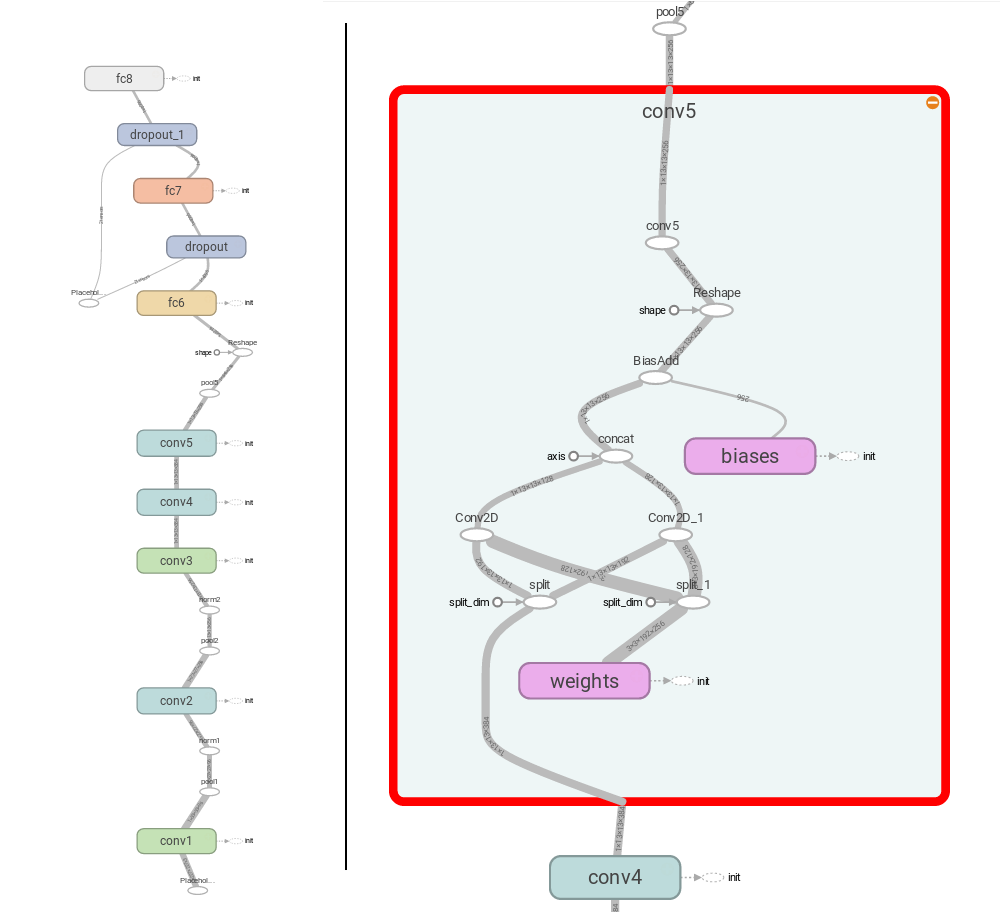
Visualization of the computational graph of Tensorboard (left) and a closer look to the conv5 layer (right), one of the layers with splitting.
Loading the pretrained weights
Okay now to the load_initial_weights function. The aim of this function is to assign the pretrained weights, stored in self.WEIGHTS_PATH, to any that that is not specified in self.SKIP_LAYER, because these are the layers we want to train from scratch. If take a look on the structure of the bvlc_alexnet.npy weights, you will notice that they come as python dictionary of lists. Each key is one of the layers and contains a list of the weights and biases. If you use the caffe-to-tensorflow function to convert weights on your own, you will get a python dictionary of dictionaries (e.g. weights[‘conv1’] is another dictionary with the keys weights and biases).
Anyway, I’ll write the function for the weights downloadable from here (dictionary of lists), were for each list item we have to check the shape of the content and then assign them to weights (length of shape > 1) or biases (length of shape == 1).
def load_initial_weights(self, session):

  # Load the weights into memory
  weights_dict = np.load(self.WEIGHTS_PATH, encoding = 'bytes').item()

  # Loop over all layer names stored in the weights dict
  for op_name in weights_dict:

    # Check if the layer is one of the layers that should be reinitialized
    if op_name not in self.SKIP_LAYER:

      with tf.variable_scope(op_name, reuse = True):

        # Loop over list of weights/biases and assign them to their corresponding tf variable
        for data in weights_dict[op_name]:

          # Biases
          if len(data.shape) == 1:

            var = tf.get_variable('biases', trainable = False)
            session.run(var.assign(data))

          # Weights
          else:

            var = tf.get_variable('weights', trainable = False)
            session.run(var.assign(data))
With this chunk of code, the AlexNet class is finished.
Test the implementation
To test if the model is implemented correctly and the weights are all assigned properly, we can create the original ImageNet model (last layer has 1000 classes) and assign the pretrained weights to all layer. I grabbed some images from the original ImageNet Database and looked at the predicted classes and here are the results.
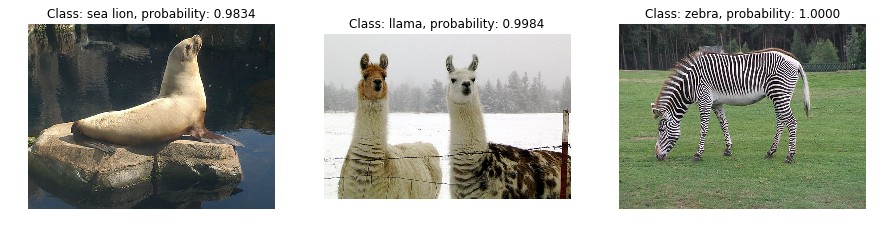
Three images taken from the ImageNet Database and tested with the implemented AlexNet class. IPython notebook to reproduce the results can be found here.
Looks good, so we can step on finally on the finetuning part.
Finetuning AlexNet
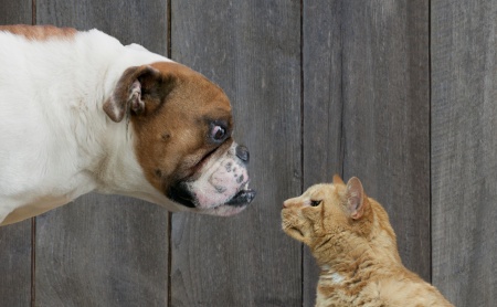
So after a long read, you finally arrived at the ‘core’-part of this blog article: Using the created AlexNet class to finetune the network onto your own data. The idea now is pretty straight-forward: We will create a model, skipping some of the last layers by passing their names in the skip_layer variable, setup loss and optimizer ops in TensorFlow, start a Session and train the network. We will setup everything with support for TensorBoard, to be able to observe the training process. For the sake of testing the finetuning routine I downloaded the train.zip file from the Kaggle Dogs vs. Cats Redux Competition.
I further splitted this images into a training, validation and test set (70/15/15) and created .txt files for each subset containing the path to the image and the class label. Having this text files I created yet another class serving as image data generator (like the one of Keras for example). I know there are smarter ways, but for another project I needed to take care of exactly how the images are loaded and preprocessed and already having this script, I simply copied it for this tutorial. The code can be founded in the github repo.
And because I personally like more scripts for educational purpose, I’ll not write the code as a callable function but as a script you should open and look at, to better understand what happens.
The configuration part
After the imports, first I define all configuration variables.
import numpy as np
import tensorflow as tf
from datetime import datetime
from alexnet import AlexNet
from datagenerator import ImageDataGenerator

# Path to the textfiles for the trainings and validation set
train_file = '/path/to/train.txt'
val_file = '/path/to/val.txt'

# Learning params
learning_rate = 0.001
num_epochs = 10
batch_size = 128

# Network params
dropout_rate = 0.5
num_classes = 2
train_layers = ['fc8', 'fc7']

# How often we want to write the tf.summary data to disk
display_step = 1

# Path for tf.summary.FileWriter and to store model checkpoints
filewriter_path = "/tmp/finetune_alexnet/dogs_vs_cats"
checkpoint_path = "/tmp/finetune_alexnet/"

# Create parent path if it doesn't exist
if not os.path.isdir(checkpoint_path): os.mkdir(checkpoint_path)
I arbitrarily chose to finetune the last two layer (fc7 and fc8). You can choose any number of the last layer depending on the size of your dataset. My choice might not be good, but here I just want to show how to select multiple layer. I left the dropout probability as in the original model, but you can change it, as well as the learning rate. Play around with this parameters and your dataset and test what will give you the best results.
Now to some TensorFlow stuff. We need to setup a few more stuff in TensorFlow before we can start training. First we need some placeholder variables for the input and labels, as well as the dropout rate (in test mode we deactivate dropout, while TensorFlow takes care of activation scaling).
x = tf.placeholder(tf.float32, [batch_size, 227, 227, 3])
y = tf.placeholder(tf.float32, [None, num_classes])
keep_prob = tf.placeholder(tf.float32)
Having this, we can create an AlexNet object and define a Variable that will point to the unscaled score of the model (last layer of the network, the fc8-layer).
# Initialize model
model = AlexNet(x, keep_prob, num_classes, train_layers)

#link variable to model output
score = model.fc8
Next comes the block of all ops we need for training the network.
# List of trainable variables of the layers we want to train
var_list = [v for v in tf.trainable_variables() if v.name.split('/')[0] in train_layers]

# Op for calculating the loss
with tf.name_scope("cross_ent"):
  loss = tf.reduce_mean(tf.nn.softmax_cross_entropy_with_logits(logits = score, labels = y))

# Train op
with tf.name_scope("train"):
  # Get gradients of all trainable variables
  gradients = tf.gradients(loss, var_list)
  gradients = list(zip(gradients, var_list))

  # Create optimizer and apply gradient descent to the trainable variables
  optimizer = tf.train.GradientDescentOptimizer(learning_rate)
  train_op = optimizer.apply_gradients(grads_and_vars=gradients)

# Add gradients to summary
for gradient, var in gradients:
  tf.summary.histogram(var.name + '/gradient', gradient)

# Add the variables we train to the summary
for var in var_list:
  tf.summary.histogram(var.name, var)

# Add the loss to summary
tf.summary.scalar('cross_entropy', loss)
This might look very difficult and complex first if you compare it to what you have to do in e.g. Keras to train a model (call .fit() on the model..) but Hey, it’s TensorFlow. The Train op could be simpler (using optimizer.minimize()) but like this, we can grab the gradients and show them in TensorBoard, which is cool, if you want to know if you gradients are passing to all layers you want to train.
Next we define an op (accuracy) for the evaluation.
# Evaluation op: Accuracy of the model
with tf.name_scope("accuracy"):
  correct_pred = tf.equal(tf.argmax(score, 1), tf.argmax(y, 1))
  accuracy = tf.reduce_mean(tf.cast(correct_pred, tf.float32))

# Add the accuracy to the summary
tf.summary.scalar('accuracy', accuracy)
Everything we miss before we can start training is to merge all the summaries together, initialize tf.FileWriter and tf.train.Saver for model checkpoints and to initialize the image generator objects.
# Merge all summaries together
merged_summary = tf.summary.merge_all()

# Initialize the FileWriter
writer = tf.summary.FileWriter(filewriter_path)

# Initialize an saver for store model checkpoints
saver = tf.train.Saver()

# Initalize the data generator seperately for the training and validation set
train_generator = ImageDataGenerator(train_file,
                                     horizontal_flip = True, shuffle = True)
val_generator = ImageDataGenerator(val_file, shuffle = False)

# Get the number of training/validation steps per epoch
train_batches_per_epoch = np.floor(train_generator.data_size / batch_size).astype(np.int16)
val_batches_per_epoch = np.floor(val_generator.data_size / batch_size).astype(np.int16)
Ok now to the trainings loop: What is the general idea? We will launch a TensorFlow-Session, initialize all variables, load the pretrained weights to all layer we don’t want to train from scratch and then loop epoch for epoch over our training step and run the training op. Every now and then we will store some summary with the FileWriter and after each epoch we will evaluate the model and save a model checkpoint. And there you go:
# Start Tensorflow session
with tf.Session() as sess:

  # Initialize all variables
  sess.run(tf.global_variables_initializer())

  # Add the model graph to TensorBoard
  writer.add_graph(sess.graph)

  # Load the pretrained weights into the non-trainable layer
  model.load_initial_weights(sess)

  print("{} Start training...".format(datetime.now()))
  print("{} Open Tensorboard at --logdir {}".format(datetime.now(),
                                                    filewriter_path))

  # Loop over number of epochs
  for epoch in range(num_epochs):

        print("{} Epoch number: {}".format(datetime.now(), epoch+1))

        step = 1

        while step < train_batches_per_epoch:

            # Get a batch of images and labels
            batch_xs, batch_ys = train_generator.next_batch(batch_size)

            # And run the training op
            sess.run(train_op, feed_dict={x: batch_xs,
                                          y: batch_ys,
                                          keep_prob: dropout_rate})

            # Generate summary with the current batch of data and write to file
            if step%display_step == 0:
                s = sess.run(merged_summary, feed_dict={x: batch_xs,
                                                        y: batch_ys,
                                                        keep_prob: 1.})
                writer.add_summary(s, epoch*train_batches_per_epoch + step)

            step += 1

        # Validate the model on the entire validation set
        print("{} Start validation".format(datetime.now()))
        test_acc = 0.
        test_count = 0
        for _ in range(val_batches_per_epoch):
            batch_tx, batch_ty = val_generator.next_batch(batch_size)
            acc = sess.run(accuracy, feed_dict={x: batch_tx,
                                                y: batch_ty,
                                                keep_prob: 1.})
            test_acc += acc
            test_count += 1
        test_acc /= test_count
        print("Validation Accuracy = {:.4f}".format(datetime.now(), test_acc))

        # Reset the file pointer of the image data generator
        val_generator.reset_pointer()
        train_generator.reset_pointer()

        print("{} Saving checkpoint of model...".format(datetime.now()))

        #save checkpoint of the model
        checkpoint_name = os.path.join(checkpoint_path, 'model_epoch'+str(epoch)+'.ckpt')
        save_path = saver.save(sess, checkpoint_name)

        print("{} Model checkpoint saved at {}".format(datetime.now(), checkpoint_name))
And we are done. Let’s have a look on the accuracy and loss diagrams of the training process. We can see, that we start of around ~50% accuracy which is reasonable and very fast reach an accuracy around 95% on the training data. The validation accuracy after the first epoch was 0.9545.
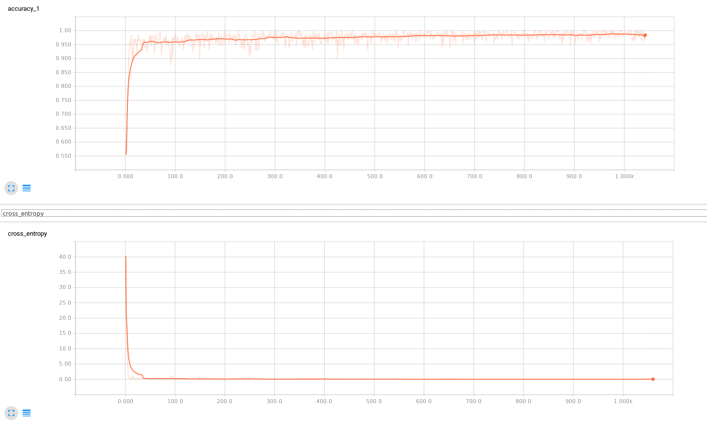
Screenshot of the training process visualized with TensorBoard. At the top is the accuracy, at the bottom the cross-entropy-loss.</a>
That the model is so fast in reaching a good accuracy rate comes from the data I chose for this exmaple: dogs and cats. The the ImageNet Dataset on which the AlexNet was originally trained already contains many different classes of dogs and cats. But anyway, there you go, finished is an universal script with which you can finetune AlexNet to any problem with your own data by just changing a few lines in the config section.
If you want to continue training from any of your checkpoints, you can just change the line of model.load_initial_weights(sess) to
# To continue training from one of your checkpoints
saver.restore(sess, "/path/to/checkpoint/model.ckpt")
Some last Note
You don’t have to use my ImageDataGenerator class to use this script (it might be badly inefficient). Just find your own way to provide batches of images and labels to the training op and implement it into the script.
If you have any further questions, feel free to ask. And again, all the code can be found on github. But note, that I updated the code, as describe at the top, to work with the new input pipeline of TensorFlow 1.12rc0. If you want to use the updated version make sure you updated your TensorFlow version.